🗺️ The Architecture of Vector Databases: How AI Stores and Searches Knowledge

In traditional software engineering, databases are built to look for exact matches. If you query an SQL database for SELECT * FROM products WHERE color = 'red', the system checks strings or integers, returning a binary “yes” or “no” match.

However, Generative AI, Large Language Models (LLMs), and computer vision operate on a completely different paradigm: semantic meaning. An AI model doesn’t care if two words share the same letters; it cares if they share the same concepts.

To bridge this gap, the modern AI stack relies on Vector Databases (like Pinecone, Milvus, Qdrant, Chroma, and pgvector). Instead of storing text tables, they store and search high-dimensional geometric spaces at sub-millisecond speeds.

In this guide, we will break down what vector databases are, the mathematics behind how they think, and write a complete implementation script in Python.

🏗️ The Vector Database Lifecycle Architecture

A vector database isn’t just a simple repository; it is a specialized engine designed to handle Approximate Nearest Neighbor (ANN) algorithms. The core pipeline is divided into three distinct operational stages:

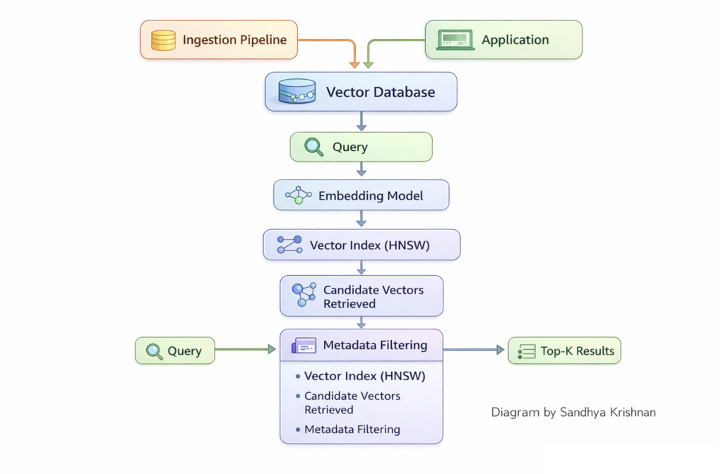
ector database retrieval pipeline architecture indexing filtering ANN. Source: sandhyakrishnan02.medium.com

Indexing (Ingestion): When raw vectors are uploaded, the database doesn’t just list them linearly. It processes them through specialized index structures (like graphs or trees) to map out geometric neighborhood zones.
Similarity Querying: When a user passes a search phrase (e.g., in a RAG system), the database converts that query into a vector, calculates the mathematical distance between it and the index, and retrieves the top $k$ nearest matches.
Metadata Filtering: Production databases allow you to combine vector search with standard filtering (e.g., “Find vectors similar to this article, but ONLY if the status metadata field equals published“).

🧠 The 3 Industry-Standard Indexing Strategies

If a database had to calculate the distance between your query vector and every single vector in a billion-row repository (a brute-force Flat Scan), the system would immediately freeze. To hit sub-millisecond response times, vector databases use Approximate Nearest Neighbor (ANN) indexing algorithms to trade a fraction of mathematical precision for massive speed gains.

1. HNSW (Hierarchical Navigable Small World)

HNSW is the gold standard for in-memory vector indexing. It organizes vectors by building a multi-layered graph, heavily inspired by the classic computer science “Skip List” data structure.

How it works: The top layers are highly sparse, containing only a few “highway” nodes with long-range connection edges. The search begins at the top, taking massive geometric leaps across the dataset. As it gets closer to the target zone, it drops down to lower, increasingly denser graph layers to execute high-precision local routing.
Pros: Blazing-fast query times (1–2ms latency) and exceptional recall accuracy.
Cons: Incredibly memory-intensive because the graph structures must live entirely in RAM.

2. IVF (Inverted File Indexing)

IVF targets memory efficiency by mapping the vector space into distinct spatial clusters using $k$-means partitioning.

How it works: The database divides the entire multi-dimensional space into thousands of Voronoi cells, each governed by a central coordinate (a centroid). When a query arrives, the database first measures distance against only the centroids. Once it identifies the top $n$ closest cells, it restricts its search exclusively to the vectors living inside those specific clusters, bypassing 99% of the remaining database.
Pros: Highly memory efficient and significantly faster to build than HNSW.
Cons: Suffer from “recall drift” if data points change frequently over time, requiring periodic re-indexing.

3. Quantization (PQ / SQ)

Quantization isn’t a standalone layout; it is a compression technique frequently layered on top of IVF index paths to slash hardware costs.

How it works: Product Quantization (PQ) takes high-dimensional vectors (e.g., 1536 floating-point columns) and breaks them down into smaller sub-vectors, compressing the raw floats into compact byte codes using a pre-calculated codebook lookup table.
Pros: Can compress database memory footprints by up to 16x.
Cons: The compression step permanently discards minor numeric details, introducing a small penalty to accuracy and recall precision.

🛠️ Step-by-Step Python Implementation with ChromaDB

Let’s write a complete Python script to load documents, embed them automatically using an open-source model, store them in a local vector database, and perform a semantic query.

Step 1: Install Dependencies

We will use Chroma, a powerful, lightweight, open-source vector database that runs entirely in-memory or persists locally.

Bash

pip install chromadb

Step 2: The Script Implementation

Create a file named vector_db_demo.py:

Python

import chromadb
from chromadb.utils import embedding_functions

# 1. Initialize the Chroma Client (Persisting data locally to disk)
client = chromadb.PersistentClient(path="./chroma_db_storage")

# 2. Select an Embedding Function
# Chroma includes a default open-source lightweight embedding model out of the box
default_ef = embedding_functions.DefaultEmbeddingFunction()

# 3. Create or Get a Collection (Equivalent to an SQL Table)
collection = client.get_or_create_collection(
    name="company_knowledge_base",
    embedding_function=default_ef,
    metadata={"hnsw:space": "cosine"} # Explicitly setting Cosine Similarity
)

# 4. Ingest Documents (Chroma handles the text-to-vector embedding generation automatically)
print("📥 Ingesting documents and generating semantic vectors...")
collection.add(
    documents=[
        "Our enterprise cloud framework provides 99.99% infrastructure uptime.",
        "The company remote work stipend allows up to $500 yearly for office hardware.",
        "For network connection failures, restart the corporate VPN software client.",
        "Annual performance review tokens are distributed every year in December."
    ],
    metadatas=[
        {"category": "tech", "author": "devops"},
        {"category": "hr", "author": "finance"},
        {"category": "tech", "author": "support"},
        {"category": "hr", "author": "management"}
    ],
    ids=["doc_1", "doc_2", "doc_3", "doc_4"]
)
print("✅ Vector indexing complete!")

# 5. Execute a Semantic Similarity Query
query_text = "How much money do we get for buying home office equipment?"
print(f"\n🔮 Querying: '{query_text}'")

results = collection.query(
    query_texts=[query_text],
    n_results=1, # Return the single closest nearest neighbor
    where={"category": "hr"} # Metadata filter condition layered on top
)

# 6. Parse and Print the Output
print("\n🎯 Top Match Found:")
print(f"📄 Content: {results['documents'][0][0]}")
print(f"📊 Distance Score: {results['distances'][0][0]:.4f}")
print(f"🏷️ Metadata: {results['metadatas'][0][0]}")

📈 The 3 Distance Metrics: How Vector DBs Measure Similarity

To find the “nearest neighbors” during the code query above, the database engine executes a mathematical distance formula between the query vector A and the stored vectors B:

Cosine Similarity: Measures the cosine of the angle between two multi-dimensional direction lines, completely ignoring the absolute length of the vectors.

\text{Cosine Similarity} = \frac{A \cdot B}{\|A\| \|B\|}

Best for: Text semantic search, where variations in document lengths shouldn’t skew the contextual meaning.

Euclidean Distance (L2): Calculates the straight-line distance between two physical points in space.

\text{Euclidean Distance} = \sqrt{\sum (A_i - B_i)^2}

Best for: Computer vision, image classification, and situations where spatial intensity matters.

Dot Product (Inner Product): Multiplies corresponding vector elements and sums the total (A · B).

Best for: Pre-normalized vectors (where vector length equals 1). It is computationally blazing fast because it bypasses expensive square root calculations.